In today's post and a few more, I will introduce you to the FEA modeling of CHT analysis in Fluent, a very common phenomenon, which is heating a room with a radiator. In the first part, we will determine the heat losses on the walls of the building with very simple dependencies and we will perform a preliminary CHT analysis of heating the room with a radiator.
 |
| 3D Temperature distribution in room with radiator and window |
In the first step, we need to describe our geometric model. It will consist of a wall, a roof and a window. We assume analytically determined heat flux (W / m2) on the upper plane (roof) and side walls. We will assume a heat transfer coefficient on the window plane with the ambient temperature outside the building. Finally, we define the constant temperature of the radiator on its outer walls. You can see the location of all the components of the model in the figure below.
 |
| Components of the geometric model |
In the next stage, we will analytically calculate heat losses in a well-insulated building. The wall of our room consists of cellular brick with a thickness of e1 = 0.24 [m] and conductivity lambda1 0.15 [W / m2K]. The facade of the building is made of polystyrene with a thickness of e2 = 0.15 [m] and conductivity of lambda2 0.042 [W / m2k]. From the first equation below, we determine the thermal resistance, so:
R = (0.24 / 0.15) + (0.15 / 0.042) = 1.6 + 3.57 = 5.17
Then we find the heat flux from equation (2):
Q = (T1 - T2) / R
where:
T1 - temperature outside the building
T2 - temperature inside the room
Q = (21 - (-12)) / 5.17 = 33 / 5.17 = 6.4 [W / m2]
Thus, the average heat flux given off by the walls of the building is 6.4 [W / m2].
In the first analysis, we will also assume this loss for the roof.
You can see the exact formulas and diagrams of the thermal resistance of the composite wall in the figure below.
More on the analytical calculations of thermal resistances, losses and other thermodynamic phenomena can be found on the website at the link below
https://myengineeringtools.com/Thermodynamics/Heat_Conduction_Wall.html
 |
| Equations for estimate heat flux over composite wall [1] |
The next step is to establish the flow solver. We choose pressure based because we deal with CHT (conjugate heat transfer) analysis. Due to the fact that we are dealing with low flow velocities, we also turn on gravity.
 |
| Pressire BAsed Solver in Ansys Fluent |
Then we turn on the energy model (heat transfer and transport) and the k-omega SSt turbulence model. We will not use the radiation model in our analysis due to low temperatures (below 60 C) and to shorten the simulation time. Radiation models considerably extend the computation time.
We establish the model of our gas as a compressible gas (ideal gas) because we want to take into account all the phenomena occurring during free convection.
 |
| Models for defined CHT Analysis in Fluent |
An important rule for compressible gases is to set the Specified Operating Density to 0. In all analyzes where ideal gas is going to be used, this setting is required. We will also use pressure outlet as a condition for gas outflow from the model - this is also a condition required for compressible gases.
 |
| Specified Operating Density in Operating Conditions - BC's defining phase |
One of the last steps is to define the boundary conditions for our model components. As I mentioned before, for the roof and side walls, we will use the same heat loss (according to our analytical calculations) of 6.4 W / m2 (red and green frames). For the window, we will assume a heat transfer coefficient of 0.9 W / m2K and an ambient temperature of -12 C (orange frame). The last condition is defined on our radiator - it will be a constant temperature of the external walls with a value of 60 C (blue frame).
 |
| BC's defined for our components in Ansys Fluent |
Then we go to the settings of our calculation solver. We set all components in the red frame to First Order, which will make our model converge faster. We set the Courant number at the level of 10. Leave the rest of the parameters unchanged.
 |
| Solver Settings and Courant Definition in Ansys Fluent |
As you can see from the charts below, we quickly stabilized the value of our defined monitor, which was the average room temperature. The residual equations also seem to be at a fairly good level.
 |
| Residuals and defined monitor curves in Ansys Fluent |
After the analysis is finished, we can check our thermal balance of the entire system. The closer it is to 0, the less gross error is in our analysis. As you can see, our balance came out at a level of less than 0.3 W, which is quite a good result with a rather poor finite element mesh and not too many solver iterations.
 |
| Fluxes report in Ansys Fluent |
Our super insulating walls, not too big room and cosmic window meant that with a not too big radiator (hot enough that you can burn yourself :)) we got a sauna.
 |
| 3D temperature distribution in room - Ansys Fluent |
The pressure based model, gravity and ideal gas gave us the opportunity to observe the movement of gas caused by its pressure change in zones of increased temperature. This is a typical phenomenon of free convection due to the adoption of a compressible gas model.

 |
| Gas flow on radiator zone - vectors in Ansys Fluent |
The last figure shows the temperature distribution in the cross-section of the model. As you can see, our heroic radiator creates a curtain that protects against ingress of cold air from the window :)
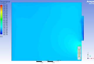 |
| Temperature distribution on corss section of the model - Ansys Fluent |
Episode 2 link below


0 Comments