In the second part of Radiator Game I would like to show you a different approach to modulating insulation on walls or heat flow resistance on windows using defined virtual layers in Ansys Fluent. In this regard, this program offers many more possibilities than the good old CFX.
 |
| Radiator Game with old construction wall |
In today's post, we will try to model the thermal resistance on the walls of the old construction and windows with one layer of glass. Usually, old, solid walls were built of red brick by way of an overlap in several construction variants. Some of them are shown in the figure below. We will be modeling the first variant for red brick with dimensions of 12x24 cm. We will simplify our model to a uniform wall of red brick with a thickness of 24 cm.
If U want more informations about evolution of building elements visit site on the link below:
https://fet.uwe.ac.uk/conweb/house_ages/elements/print.htm
 |
| Wall construction from red brick in late 19th century |
In the first stage, we need to define the material properties of red brick and glass. Below you can see the exact parameters I used for the simulation.
 |
| Materials properties defined for simulation |
The second and key stage of modeling is to define the virtual layers of the model on the faces of the geometry. The general assumption behind the definition of virtual layers is to define boundary conditions based on the temperature outside these layers. And so for the side walls (walls) and the roof, we define the external temperature at the level of -12 C. In the material name option, we choose red brick. Finally, we set the wall thickness - in our case it will be 0.24 [m]. We leave the rest of the options unchanged on these two boundary conditions.
Similarly, we define a boundary condition for the window. In material name, we choose glass, set the layer thickness to 0.008 [m] and assume the external temperature at -12 C.
We leave the boundary condition for the radiator unchanged, as in the previous part of Radiator Game.
 |
| BC's for RAdiator Game part 2 - virtual layers |
As you can see in the picture below, the room is Spartan :). It's cold and the temperature goes even below 0.
 |
| 3D Temperature Distribution in Room for Virtual Layers Method in Ansys Fluent |
The temperature in most of the room's space ranges from -5 C to 0 C.
 |
| Temperature distribution on cross section of the room for 12 ranges |
If we increase the resolution of the decomposition to 120 ranges, the operation of our radiator can be clearly seen.
 |
| Temperature distribution on cross section of the room for 120 ranges |
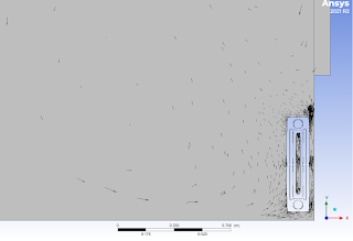
Below you can see the distribution of air movement in the cross-section of the room caused by mixing of warm air with cold air from the radiator.
 |
| Distribution of flow direction of air in corsso section of the room - Ansys Fluent |
P.S
I also wanted to present the solver results. You can see that the level of partial equations reaches decent values. The defined monitor has also reached stable values without major fluctuations.
 |
| Residuals and defined Monitor after 225 iterations in Ansys Fluent |
Episode 1 link below


0 Comments