In today's post, I would like to show you a tutorial on how to model a bullet flight in Ansys Fluent. Due to the earlier post where the bullet was modeled in the SimScale software, it will be an interesting comparison, especially when it comes to gas velocity distributions.
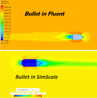 |
| Comparision of velocity distribution on Bullet Fly Fluent/ SimScale |
In the first step, we choose the Density Based solver which is dedicated to modeling gases at high speeds above Mach 0.3. We do not take gravity into account as its influence will be negligible at such high gas velocities (over 570 m / s).
 |
| Density Based Solver for high speed analysis in Fluent |
As for the turbulence model, we leave the k-omega universal SST model as default. We leave all settings of this model in the default position. If you want to learn more about what model of turbulence is adequate to your modeled phenomenon, it is worth using the ANSYS tutorial or reading the thread below.
discussion over turbulence models on high speed
 |
| Turbulence model in Ansys Fluent |
With the Density Based solver and to simplify our simulation, we choose the linear gas model (air). Below you can see the defined properties of the gas.
 |
| Properties of linear gas model in Ansys Fluent |
The next step is to define the boundary conditions in our model. We assume Velocity Inlet with a speed of 570 m / s. As an outlet, we define an absolute pressure of 1 atm. The boundary conditions are presented below. Remember that if you leave all other faces of the model in the default position, then friction and considerable turbulence will occur on the external walls of the model. If you want to speed up the convergence of the partial equations, choose the Wall Slip option.
 |
| BC's on Fluent |
An important element of the analysis (especially steady state) is the definition of monitors. In addition to the observations of Residuals, it is worth defining the monitor on a selected plane of the model to verify whether we obtain stabilization of the calculated values. In our case, we define the average speed variable to Outlet. After this value stabilizes, we will know that we are striving for the convergence of our analysis.
 |
| Average Velocity on Outlet - defined monitor in Ansys Fluent |
In the next stage, we define how detailed our analysis should be, determining the maximum Residuals errors. In our case, we leave all Residuals at their default position of 0.001.
 |
| Residuals definition on Ansys Fluent |
Below you can see the velocity vector distributions on the cross section of the model and the turbulent kinetic energy and pressure distributions.
 |
| Velocity vectors on corsso section in Ansys Fluent |


0 Comments