It often happens that we want to do a coupled analysis consisting of two CFD and Structural modules. The purpose of FSI analyzes is to set the thermal conditions that came out from CFD simulation to the Structural analysis as boundary conditions. In the module for mechanical calculations itself, we cannot set a heterogeneous temperature profile, therefore it is necessary to perform two analyzes in these cases as FSI. A very common problem in this type of analysis is a bad transfer of thermal conditions to the Structural module. The distribution of values is not the same as what we came out with CFD. Therefore, in these cases, you can simplify the analysis by adding one more Transient Thermal module from which the transfer of temperature distributions is burdened with a much smaller error.
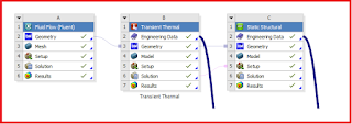 |
| III stages for simplify FSI case |
It is known that this will not translate into increasing the precision of calculations, but if we do not have too high requirements, we want to determine and verify something fairly quickly, the path that I will show you may be just perfect for this.
First, you need to do CFD analysis, preferably in Fluent. Of course, you can skip this step if you decide that all conditions will be accurately mapped in Transient Thermal. But sticking to this three-step path - after performing the thermal analysis, we can export the results from the element you are interested in, which is the heat source (e.g. average temperature from solid domain). Of course you can write your own user define function thanks to which you will be able to extract the results that interest you the most (Variable, Expression). Later, you export the results from the graph window in Postprocessing using the Export key (red frame).
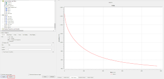 |
| How to export results in Postprocessing |
When you export your results to a CSV file later, you need to use a spreadsheet (excel, for example) for correct data processing (separating columns and rows, replacing a period with a comma, etc.).
After processing, you can copy the data (time and temperature) to the Temperature boundary condition in Transient Thermal. With this method, you will make the boundary condition dependent on time, thanks to which you will approximate the total heat flux that will be transferred to the rest of the cold elements.
 |
| Example of imported temperature profile in Transient Thermal |
The figure above shows an example of a temperature profile imported to Transient Thermal. You paste the data directly into the table. Then you will generate a graph corresponding to your profile. Of course, by defining the analysis time, you can only simulate a given segment of the boundary condition that you imported into tansient thermal.After performing the thermal analysis in Transient Thermal, you need to connect the Solution block from this analysis to the Setup block in Static Structural. Thanks to this, you will be able to set a boundary condition in the form of temperature distribution on the analyzed elements in the structural analysis.
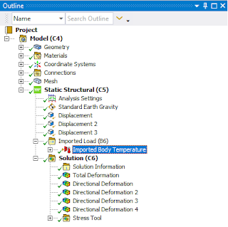 |
| Example of imported load (temperature profile) in Static Structural |
After opening the Static Structural module, the Import Load option will appear in the tree. In this function you will be able to import the results from the previous analysis. You can select the entire model for mapping, but you might as well define conditions on only those elements that you select. And that's all at this point you can perform a mechanical analysis supplemented with thermal conditions.
Of course, You should remember to define the material properties correct at all three stages of modeling. Especially if you are analyzing stresses and deformations, it is worth implementing the hardening curve depending on the temperature.


0 Comments