Another tutorial I would like to introduce to you is the CHT analysis. It is one of the most commonly used types of simulation. In SimScale, you can go through all the phases of Conjugate Heat Transfer (CHT) modeling in a few simple steps.
 |
| Conjugate Heat Transfer (CHT) used in "Nozzle Game" |
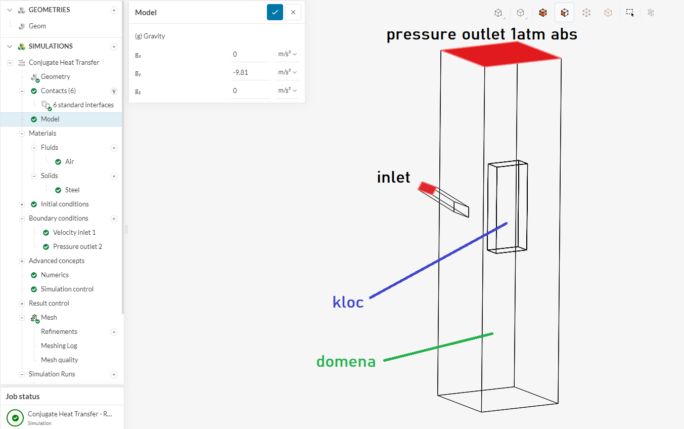
The first step is to load the geometric model into SimScale. In the contrast to the previous tutorial, here we will deal with two types of domains - a solid (kloc) and a gas domain (domena). At the beginning, we define the type of analysis (in our case, transient) and the turbulence model (SST k-omega). Then we assume gravity, which is very important in the case of modeling compressible gases (modeling of hydrostatic phenomena) (Image below).
 |
| Model used in CHT Analysis |
The contact between a solid and a liquid in a correctly built geometric model will be defined automatically in SimScale (contacts 6 - a cube). Then we define the materials. In the gas domain, it will be air as an ideal gas, compressible gas). For kloc, we define steel with constant thermal properties that do not change as a function of temperature (of course, in the SimScale program it is possible to define User Defined Function - UDF).
 |
| Steel and Air defined in CHT Analysis |
As for the boundary conditions, there will be two in our model. For Inlet it will be a velocity along the X axis of 30 m /s and a gas temperature of 120 C. As the output of the model, we will set a pressure Outlet with a value of 1 atm ABS.
 |
| BC's in CHT Analysis |
Residuals and relaxation factors we are leaving on default values (see image below).
 |
| Residuals and relaxation factors in CHT Analysis |
In the next step, we define the total analysis time (end time - 12 s) and the size of the time step (Delta T - 0.5 s). We switch the adjustable time step to false because we want the size of our time step not to be adaptive. We also define Write Interval as 6. Then out of 24 time steps (12 / 0.5 = 24) every 6 will be written to the postprocessor. The entire configuration can be seen in the figure below.
 |
| Defined Tme Step Size and End Time in CHT Analysis |
The last step before initiating the analysis is the discretization of the geometric model. We leave Sizing in the Automatic option at 5 value and the Algorithm in standard mode. After meshing we get 200k nodes and 400k elements (all configuration and statistics are shown in the picture below).
 |
| Discretized model for CHT Analysis |
Below temperature distribution on cross section of the model is presented at time 12 s.
 |
| Cross-section Temperature distribution on the CHT Analysis |
Below velocity distribution on cross section of the model is presented at time 12 s.
 |
| Cross-section velocity distribution on the CHT Analysis |
Four velocity distributions on different time steps.
 |
| Four time steps velocity distribution on CHT Analysis |
Interesting option of isosurface plot. Thanks to this option, you can easily present the velocity distribution in the model in the 3D spatial mode. With the Iso-value we define the minimum velocity to be displayed with this option (> 10 m / s).
 |
| Iso-surface option in postprocessing - CHT Analysis |
Another interesting option is IsoVolume. With this option, we can define a finite volume in 3D with a given variable, e.g. temperature. We define the values in the MIN-MAX range.
 |
| Iso-Volume option in CHT Analysis |
My proposal in the next versions of SimScale is to add an option, e.g. to Cutting Plane, of the solid / plane selection function on which the variable values will be plotted. This will greatly facilitate the work in the result processing mode and the same options will be logically arranged both in the pre and post processor stages.
 |
| Propostion of additional cutting plane function (CHT Analysis) |


Comments
Post a Comment